Probabilistic Forecasts#
Conventional VARs produce point forecasts. A Bayesian VAR produces a full posterior predictive distribution over future paths. This means every forecast comes with calibrated uncertainty — wide bands when the model is unsure, narrow when the data are informative.
That uncertainty has two sources: the model’s coefficients are only estimated, and the system is hit by a fresh random shock every period. forecast() includes both by default. The section below shows why leaving the shocks out — as much VAR tooling implicitly does — understates uncertainty, badly so at short horizons.
import matplotlib.pyplot as plt
import numpy as np
import pandas as pd
from qc_core import plotting

from impulso import VAR, VARData
from impulso.samplers import NUTSSampler

plotting.use_ledger_style()
Setup#
We repeat the data-generating process from the quickstart tutorial. The DGP is a VAR(1) with three macro variables — GDP growth, inflation, and an interest rate. If you’ve already worked through that notebook, the setup code below will be familiar.
rng = np.random.default_rng(42)
T = 200
n_vars = 3

A_true = np.array([
    [0.6, 0.0, -0.1],
    [0.2, 0.5, 0.0],
    [0.0, 0.15, 0.4],
])

y = np.zeros((T, n_vars))
for t in range(1, T):
    y[t] = A_true @ y[t - 1] + rng.standard_normal(n_vars) * 0.1

index = pd.date_range("2000-01-01", periods=T, freq="QS")
data = VARData(endog=y, endog_names=["gdp_growth", "inflation", "rate"], index=index)

sampler = NUTSSampler(draws=500, tune=500, chains=2, cores=1, random_seed=42)
fitted = VAR(lags=1, prior="minnesota").fit(data, sampler=sampler)
fitted
FittedVAR(n_lags=1, data=VARData(endog_names=['gdp_growth', 'inflation', 'rate'], exog_names=None), var_names=['gdp_growth', 'inflation', 'rate'], volatility=Constant(name='constant', is_time_varying=False, sigma_sd_beta=2.5, tril_offdiag_sigma=0.5, innovation_scale_priors=None), error_dist=Gaussian(name='gaussian', is_heavy_tailed=False))
Point forecasts#
Call .forecast(steps=8) to produce an 8-step-ahead forecast. The result is a ForecastResult object that holds the full posterior predictive draws. The .median() method extracts the central tendency — the posterior median at each horizon.
fcast = fitted.forecast(steps=8)
fcast.median()
| gdp_growth | inflation | rate | |
|---|---|---|---|
| 0 | -0.013656 | 0.069318 | -0.049242 |
| 1 | -0.009944 | 0.024330 | -0.026080 |
| 2 | -0.004302 | 0.017727 | -0.018600 |
| 3 | -0.007068 | 0.006051 | -0.003699 |
| 4 | -0.008110 | 0.005138 | 0.001691 |
| 5 | -0.005319 | -0.009955 | 0.008959 |
| 6 | 0.010854 | -0.005531 | 0.006454 |
| 7 | 0.008893 | -0.005889 | -0.000054 |
Each row is a forecast horizon (1 through 8 quarters ahead). The values converge toward the unconditional mean of the process as the horizon increases — a hallmark of stationary VARs.
Credible intervals#
The .hdi() method computes the highest density interval at a given probability level. An 89% HDI means 89% of the posterior forecast mass falls within these bounds. We use 89% rather than 95% following the ArviZ convention — it avoids the false precision of round numbers.
Lower bounds:
   gdp_growth  inflation      rate
0   -0.183634  -0.091444 -0.209430
1   -0.208727  -0.137839 -0.188643
2   -0.227878  -0.198712 -0.202413
3   -0.226280  -0.209894 -0.201309
4   -0.233076  -0.196196 -0.203606
5   -0.221991  -0.214922 -0.179407
6   -0.237167  -0.213869 -0.185464
7   -0.220469  -0.230407 -0.199401

Upper bounds:
   gdp_growth  inflation      rate
0    0.145973   0.236012  0.103524
1    0.163294   0.231591  0.149456
2    0.186111   0.202648  0.165903
3    0.211942   0.197173  0.179435
4    0.208289   0.216072  0.171125
5    0.218719   0.200471  0.187251
6    0.198353   0.210128  0.184098
7    0.220510   0.199759  0.182523
The intervals widen at longer horizons. This is expected: two forces compound over time — the random shocks hitting the system accumulate, and parameter uncertainty propagates forward as each forecast step feeds into the next.
Visualise the forecast#
The .plot() method produces a fan chart showing the median forecast with shaded credible bands for each variable.
fig = fcast.plot()
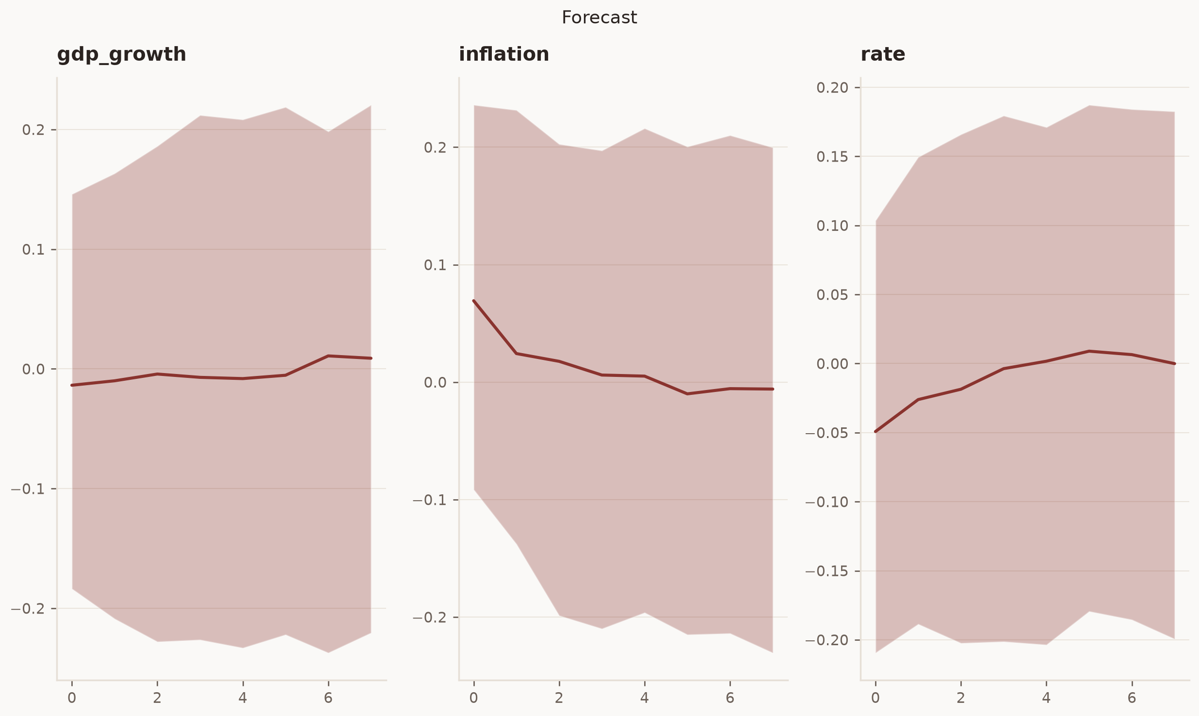
The fan chart shows the posterior median (line) and 89% HDI (shaded region) for each variable. The bands widen at longer horizons, reflecting compounding uncertainty. GDP growth and the interest rate show the widest bands, consistent with their stronger cross-variable dependencies in the DGP.
What the bands include#
The forecast above is a genuine posterior predictive distribution: it composes parameter uncertainty (the coefficients are estimated, not known) with shock uncertainty (each future period draws a fresh innovation). This is the default — include_shock_uncertainty=True.
Setting include_shock_uncertainty=False switches the shocks off and propagates only the posterior over conditional-mean paths. The result is a distribution over what the model expects to happen, not over what will happen. It is the right object for scenario mechanics, but it is not a predictive distribution — and reporting it as one is a common way to understate forecast uncertainty. Pass seed in density mode to make the drawn shocks reproducible.
mean_fcast = fitted.forecast(steps=8, include_shock_uncertainty=False)
density_fcast = fitted.forecast(steps=8, include_shock_uncertainty=True, seed=42)

mean_hdi = mean_fcast.hdi(prob=0.89)
density_hdi = density_fcast.hdi(prob=0.89)
Plotting both 89% bands on the same axes shows the gap. The narrow inner band is parameter uncertainty alone; the wider band is the full predictive.
horizons = range(1, 9)
fig, axes = plt.subplots(1, n_vars, figsize=(12, 4), squeeze=False)

for i, name in enumerate(data.endog_names):
    ax = axes[0][i]
    med = density_fcast.median()[name].values
    ax.fill_between(
        horizons, density_hdi.lower[name], density_hdi.upper[name],
        alpha=0.25, color="C0", label="full predictive",
    )
    ax.fill_between(
        horizons, mean_hdi.lower[name], mean_hdi.upper[name],
        alpha=0.5, color="C1", label="parameter only",
    )
    ax.plot(horizons, med, color=plotting.COLORS.ink, lw=1)
    plotting.serif_title(name, ax)
    ax.set_xlabel("horizon")

_ = plotting.legend_below(axes[0][0], per_row=2)
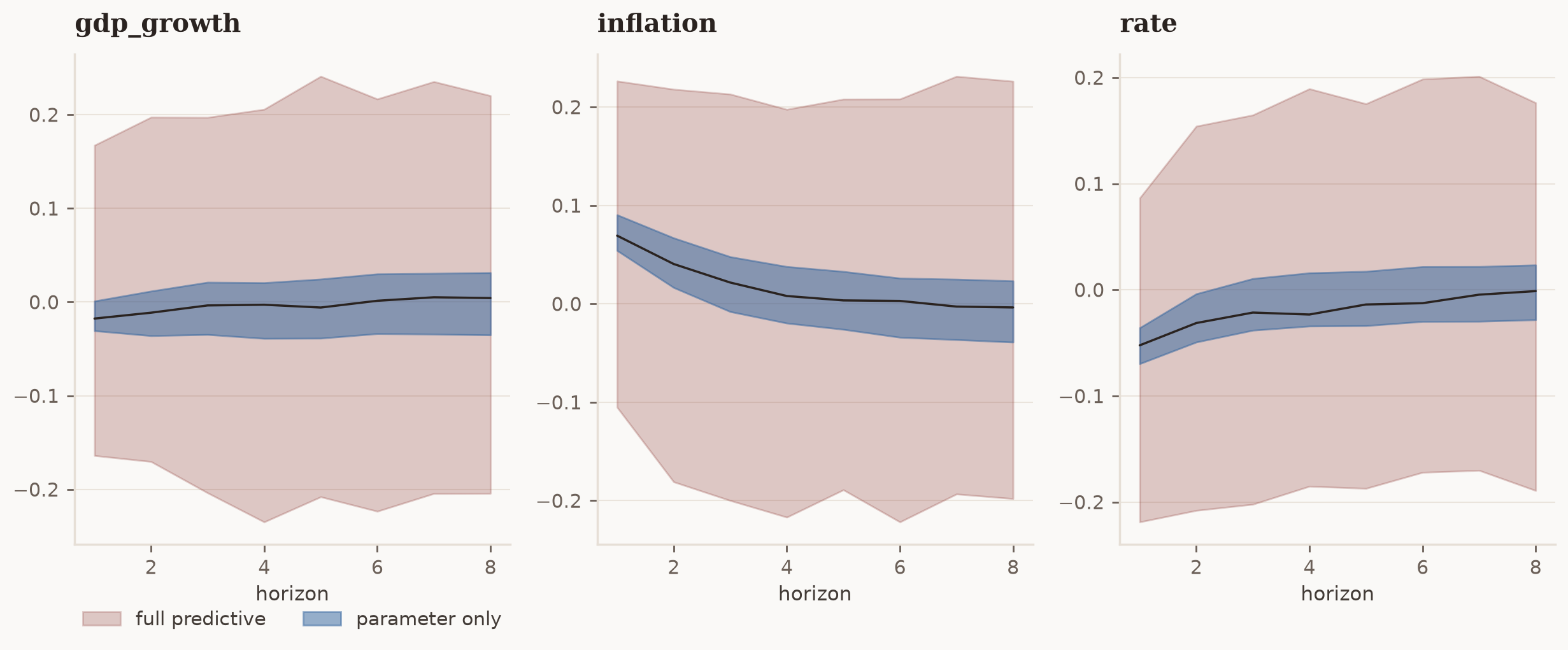
The understatement is worst at the shortest horizons. At h=1, parameter uncertainty is small — the data pin the coefficients down — so a mean-only band is almost invisible, yet the true one-step forecast still carries the full shock variance. The ratio of band widths makes this concrete:
width_mean = mean_hdi.upper - mean_hdi.lower
width_density = density_hdi.upper - density_hdi.lower

ratio = (width_density / width_mean).round(1)
ratio.index = range(1, 9)
ratio.index.name = "horizon"
ratio
| gdp_growth | inflation | rate | |
|---|---|---|---|
| horizon | |||
| 1 | 10.4 | 9.1 | 9.0 |
| 2 | 7.7 | 7.9 | 8.0 |
| 3 | 7.2 | 7.4 | 7.5 |
| 4 | 7.4 | 7.2 | 7.5 |
| 5 | 7.1 | 6.7 | 7.1 |
| 6 | 6.9 | 7.2 | 7.2 |
| 7 | 6.8 | 6.9 | 7.2 |
| 8 | 6.4 | 6.8 | 7.1 |
Each entry is how many times wider the honest band is than the parameter-only band. The multiple is largest at h=1 and shrinks as parameter uncertainty grows into the total — the opposite of the intuition that near-term forecasts are the certain ones.
Tidy export#
For downstream analysis or dashboarding, .to_dataframe() returns the median forecast in a tidy DataFrame format.
fcast.to_dataframe()
| gdp_growth | inflation | rate | |
|---|---|---|---|
| step | |||
| 0 | -0.013656 | 0.069318 | -0.049242 |
| 1 | -0.009944 | 0.024330 | -0.026080 |
| 2 | -0.004302 | 0.017727 | -0.018600 |
| 3 | -0.007068 | 0.006051 | -0.003699 |
| 4 | -0.008110 | 0.005138 | 0.001691 |
| 5 | -0.005319 | -0.009955 | 0.008959 |
| 6 | 0.010854 | -0.005531 | 0.006454 |
| 7 | 0.008893 | -0.005889 | -0.000054 |
Summary#
Bayesian VAR forecasts provide more than point predictions. The full posterior predictive distribution lets you quantify and communicate forecast uncertainty honestly. For structural questions — what happens to inflation when the central bank raises rates? — see the Structural Analysis tutorial.